How we tune a GPU pipeline in an agentic world

TL;DR from the author

”The interesting part of this story is how little we added to get to the result. A pipeline small enough to see, a ceiling computed before the first experiment, and a coding agent that spent the day proving ideas wrong against a five-minute benchmark, one change per run. The human's job was not to have the ideas. It was to keep the code simple while the number climbed.”

Embedding a corpus is, on paper, one of the simplest programs you can write. Load a model, hand it text, get vectors back, write them down. You could sketch it on a napkin in a minute.

Those vectors are the representation of the web that a search API for AI actually retrieves against. We run the job over the output of a crawler that fetches billions of pages a day. Throughput is how often that representation can be rebuilt, and the number that matters is how many tokens per second you get out of a GPU you are already paying for.

This post is about a day in June when we took that job from about 37,000 tokens per second per GPU to a bit over 200,000, and about where the difficulty actually was. Almost none of it was in the model, and almost none of it was in the chip. It was in the pipeline around them, and in whether we could see that pipeline at all.

The path this post takes

We go from the old design down to the day itself, in four moves:

1. Why the old system could not be improved. Embeddings ran in Spark behind a hosted API, which left three knobs and no way to compute a ceiling.
2. The arithmetic that prices the job. A five-minute calculation (the roofline) that said we were using about 4% of the chip.
3. How we spent the day. A coding agent, a benchmark cheap enough to run twenty-five times, and one change per run.
4. Where we stopped, and what we kept. 25% utilisation, a pipeline small enough to read, and a corpus that now re-embeds in a fifth of the time.

Why the old design could not be tuned

Before any of this, embeddings were computed inside a Spark job that called a hosted API. That was a reasonable design at that stage. The model was somebody else's problem, Spark already ran the rest of the lakehouse, and the vectors came out correct on a schedule.

It was also a design with almost no surface to work on. Enumerate the levers honestly and you get three: how many texts you put in a request, how many requests you keep in flight, and how many partitions Spark splits the input into. Everything that actually determines throughput (which GPU is serving you, which inference engine, its batching policy, its precision) sits behind an HTTP call you cannot see through. You cannot compute a ceiling against hardware you cannot name, so last week's tokens-per-second is the only comparison you have. That is how a team can sit at 4% of the chip and think they are finished.

The inference on the far side of that call was probably fine. The service was running the same class of engine we run today, on hardware at least as good as ours. We were never short of fast math. We were short of any way to see the pipeline around it, which is where most of the throughput in a job like this actually lives.

Spark made that worse, and not because Spark is a bad system. It is a serious distributed engine built for joins over huge tables, and you pay for that in full (executors, heaps, skew, shuffle, a scheduler with its own opinions about parallelism) even when the job is "send text, wait, get numbers back." On top of that, Spark was deciding how much work to put in flight while the vendor's API was deciding, on a different timescale, how much capacity to answer with. Two distributed systems, nested, neither aware of the other.

Spark's instrumentation, which is genuinely good, then reports the wrong layer: stages, task durations, GC pauses. The bottleneck we care about is a GPU sitting idle, and from where Spark is standing a worker blocked on an HTTP call is simply a task that is taking a while. Throughput would move, and we would be left with two or three explanations and no way to pick one.

The frame we use for GPU work is Formula One. An F1 car makes its numbers on a track that has been swept and closed. Put the same car on a public road and it goes slower than a hatchback, while costing a thousand times more to sit there. Treat the H100 as the car and everything else in the pipeline as the road, and Spark calling a hosted API is not a road you would put that car on. It is not even your road.

So the first move was a rewrite we controlled end to end: pull the weights, run them on our own GPUs, in a few hundred lines of Python small enough to read in one sitting. We did not do this because we expected the new version to be fast. We did it because it was the first version where "how fast could this be?" was a question with an answer.

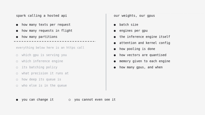
Under the old design, three things you can change and six you cannot even see. Under the new one, eight things you can change and nothing hidden.

The systems that are hardest to speed up are usually already so complex, or so far behind an abstraction, that there is no room to try anything. "I would like to replace a working system so that I can find out whether it is slow" is a difficult sentence in a planning meeting. The 6× in this post is what that rewrite paid for.

Once we owned the GPUs, we wrote the most boring thing that could work: a Ray Data pipeline, one operator, a pool of GPU workers, and inside each worker a small encoder called the obvious way through Hugging Face, with every constant a default or a guess. Starting there is deliberate. You get a system whose behaviour you can predict, so that when you change one thing and the number moves, you know which thing moved it.

It worked on the first serious run. The vectors matched the reference implementation, and by every criterion we had written down the job was done. It was also using about 4% of the hardware, which we only knew because we could finally do the arithmetic.

The roofline, and what it told us

You should run this calculation before you touch a GPU pipeline. It takes five minutes, it needs two numbers off the datasheet and one about your model, and it tells you whether the work in front of you is worth doing at all.

The roofline asks whether, for this job, the machine is limited by how fast it can compute or by how fast it can move data:

attainable FLOP/s = min( peak FLOP/s , arithmetic intensity × peak bandwidth )

A FLOP is one math operation. Arithmetic intensity is the amount of useful math you do per byte moved through memory. Every chip has a ridge where those two limits meet, which is just peak compute divided by peak bandwidth. Below the ridge you are waiting on memory, and a faster GPU will not help. Above it you are waiting on math, and the only job is keeping the chip fed. For an H100, 989 TFLOP/s of dense bf16 against 3.35 TB/s of memory bandwidth puts that crossover around 295 FLOP per byte.

The workload side is one constant. A forward pass costs about two FLOPs per parameter per token, so if you multiply by the throughput you are actually seeing and divide by the chip's peak, you get model FLOPs utilisation (MFU): the fraction of the chip you are really using, in a form you can compare across models and hardware. Ours came to a little over 4%, which is the F1 car sitting in city traffic.

Nobody ever reaches 989 TFLOP/s, so measuring against it can look unfair. Peak is a track number, and its only job is to be a fixed reference. The distance between your number and it is how much of the road is still obstacle.

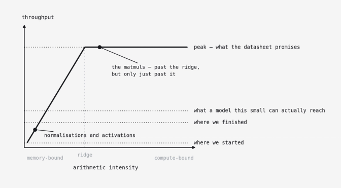
The sloped line and the flat line are the machine. Where a kernel sits along the bottom decides which of the two it runs into. The work in this post is the vertical gap between where we started and where a model this small can actually reach.

The roofline did not tell us which line of code was wrong. What it told us is that the 96% we were leaving on the floor was not physics, not memory bandwidth, not the shape of the model, and not anything a bigger GPU would fix. The GPU was simply not computing for most of the time. That is a different investigation from "we are bandwidth-bound," and a much more useful one to be in.

It also told us whether to spend the day. If the arithmetic had come back at 80% of what the chip can do, the right move would have been to close the laptop. At 4% there was a twenty-fold argument for trying, and that decision took five minutes.

How we spent the day

We did not hand-tune the pipeline. We handed it to a coding agent and spent the day approving experiments rather than running them.

That only works if a bad idea is cheap to catch. An agent that proposes optimisations in prose is not worth much, however good the proposals sound, because a proposal you cannot settle is just an argument. The expensive part of this work has never been coming up with ideas. It is the round trip between having one and knowing whether it helped, and if you compress that round trip, being wrong stops costing the afternoon.

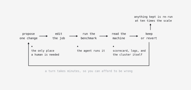
A human is needed only at the first step. The agent edits the job, runs the benchmark, and reads the scorecard, the logs, and the cluster. Anything kept is re-run at ten times the scale.

The loop also only works if a change has a readable effect. Point an agent at the old Spark job and it will generate plenty of activity and nothing you can attribute, which is why the rewrite had to come first. Given a system you can actually see, the thing to build next is not a better prompt and not a cleverer model driving the agent. It is the benchmark, because everything the loop produces is downstream of whether you can believe its verdicts and how many of them you can afford per hour.

Ours needed four properties at once.

One number, printed by the program itself

At the end of every run the job printed its own scorecard:

Done in 276.7s, processed 100,000 document rows end-to-end tok/s : 652,000

The agent never had to instrument anything, scrape a dashboard, or decide what to measure. The objective was three lines of stdout, the same three lines every run, so a result at 9am was comparable with a result at 5pm. That small decision is the one the rest of the day hung on.

Cheap enough to run twenty times, with a slower test behind it

We used a fixed table of 100,000 documents, five or six minutes a run, and did about twenty-five over the day including failures. Past about ten minutes you start batching changes to save runs, and the moment you batch changes you can no longer tell which one did what.

The cheap benchmark also lies, and you should assume yours does too. Ours had a slightly heavier document mix than production and a runtime too short to hide engine startup, which can flatter some changes and punish others. Anything that looked like a winner was therefore re-run at ten times the scale before we counted it, and more than one "win" died there.

The agent runs the jobs and reads the machine without asking

It submitted with ray job submit, tailed the logs, and killed runs that had clearly gone wrong. We never ran a command. The scorecard tells you something is wrong without telling you what, because the explanation lives one level down (utilisation, memory, per-worker progress), so the agent has to be able to go and get those numbers rather than guess from logs or wait for a person to describe them. Ours had a shell on the cluster and pulled them itself. I worked alongside it the whole time, but as a second opinion on the same data, not as the pipe carrying it. The constraint on this kind of work is context, and the fix is access to the instruments, not a better prompt.

The most useful thing that layer showed us was not a bottleneck. GPU memory sat nearly empty from morning to night. An encoder has no growing cache of past tokens, so there is nothing to fill that memory with, which means empty memory here is unused capacity you are paying for rather than a symptom to chase. That is also why several copies of the engine fit on one card. The right response is fewer, busier GPUs, not bigger batches to occupy the space. An agent watching only the throughput number would have spent the afternoon trying to fill it.

One variable per run

This was the only rule we had to learn the expensive way. Early in the day the agent shipped three plausible CPU-side changes in a single commit, throughput dropped by 2.6×, and it took four more runs to establish which of the three had done it. After that, unprompted, it started proposing changes one at a time and writing its own caveats into each analysis. Restricting the loop to one variable did not slow it down. It is what made the output worth believing.

What moved the number

Of twenty-five runs, five survived, and every one of them stopped the GPU waiting on the CPU, the single category the roofline had pointed at. The agent supplied the ideas. Agreeing on what each result meant was the harder part.

The structural change came first. Replacing eager Hugging Face forward passes with a vLLM engine in pooling mode bought continuous batching, FlashAttention, and CUDA graphs in a single import. Same weights, different code executing them. Everything after that was pipeline work.

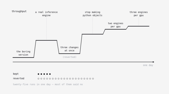
Twenty-five runs in one day. The dip is three changes shipped at once, then reverted. The steps that survived stopped the GPU waiting on the CPU.

The useful thing in that staircase is not the individual steps but their common mechanism. Almost nothing that worked made the GPU faster. What worked stopped the GPU waiting on the CPU: a line of Python deleted in one place, three copies of the engine sharing a card in another. That is exactly what the roofline had said first thing in the morning, when it put the missing 96% in software rather than in physics.

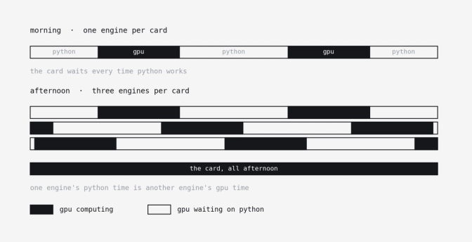
Morning: the GPU waits on Python. Afternoon: three engines keep it fed while Python works for one of them.

Without the ceiling, twenty-five experiments is enough rope to wander for a week. With it, the day became a search inside one category, and everything outside that category could be dismissed without spending a run. The order of operations is the part worth copying: compute the ceiling, let it tell you which class of change is eligible, and only then start experimenting. Most performance write-ups go the other way, which is why they read as a list of things somebody tried.

Every good idea that day came from the agent. We did not supply the hypotheses and have a machine type them up. Plenty of the ideas were bad, which matters less than it sounds when a verdict costs five minutes. The example we still bring up had a clean argument behind it: the hardware supports a faster numeric format, the model is small enough that the lost precision cannot matter, and the arithmetic checks out at every step. It measured slower, because converting formats and giving up well-tuned code paths cost more than the theoretical gain. Nothing about that was knowable from a desk.

Wrong ideas were cheap. Wrong conclusions were not. An agent will read a result and tell you what it means, fluently and with confidence, and that reading is usually sensible, sometimes debatable, and occasionally wrong in a way that would send the next three experiments down a dead end. Its arithmetic was reliable all day. What a given measurement implied about the system is a different kind of claim.

Two parties only converge if they agree on where they are now and where they should be going. The benchmark is a shared answer to the first, identical whoever reads it. The roofline is a shared answer to the second. Drop either one and the loop still looks busy: two people holding different pictures of the system will produce plausible, well-argued, incompatible next steps for as long as you let them, and the number will wander.

That is why a person stays in the loop, and it is not to fetch information the agent cannot reach. It is to look at the same data with different assumptions.

A loop like this will keep producing candidates for as long as you let it run, which raises a question the loop itself cannot answer: how do you know when you are done?

Knowing when to stop

By late afternoon we were at about 25% MFU, up from 4%. The obvious question is whether to keep going, and that is exactly where teams burn a second week. You stop when you can show that the thing you were fixing (the GPU sitting idle) is actually fixed.

A sixty-second profile of a worker in steady state settled it. The GPU is busy essentially all of the time, so there is no starvation left. Memory bandwidth is nowhere near saturated. The link back to the host runs an order of magnitude below capacity, so moving results off the card is not the constraint either. The remaining gap is therefore not idle time, which leaves a contradiction: the GPU looks 100% busy, and we are only doing 25% of the math it is rated for.

Those two numbers can both be true. nvidia-smi calls a chip busy when any thread is sitting on it. It says nothing about whether the units that do the heavy matrix math are actually multiplying. A GPU running the cheap leftover operations (normalisations, activations, residual adds) reports a full chip while doing almost no floating-point work.

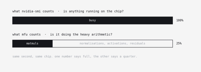
nvidia-smi counts occupancy. MFU counts arithmetic. A chip doing normalisations all afternoon reports 100% and does almost no math.

A small model is a harder machine to saturate than a big one. The peak numbers on the datasheet assume you are feeding the chip large matrices. This model's matrices are not, so the ceiling that applies to us is not the one printed on the box, and no amount of pipeline work will move it.

"GPU 100% busy" here means the road is clear, and clearing it is the entire content of this post. What is left is the car. Getting meaningfully further means kernel fusion, a custom on-GPU pooler, or a wider model, all of which are projects rather than knobs. Knowing that is what let us close the laptop instead of spending another week discovering it one failed experiment at a time.

What we ended up owning

The word "simple" gets used for two opposite things in engineering arguments. There is simple as unfinished: the boring first version, written before you understand the problem. And there is simple as refined: the smallest system that actually does the job, arrived at once you understand the problem well enough to stop over-solving it. We started with the first. The day was aimed at the second.

The champion pipeline is simple in that second sense, even though a parts list makes it sound like the opposite. It runs a continuous-batching inference engine with custom kernels and compiled GPU graphs, three copies per card, inside a distributed streaming framework with an autoscaling actor pool, which is far more machinery than there ever was in the Spark job we deleted. The part we own is a few hundred lines one person can read in a sitting. The question is not how much complexity exists in the system, but how much of it you have to hold in your head.

vLLM is by some distance the most complicated thing in the pipeline, and taking it cost one import and a block of configuration. Continuous batching, FlashAttention, CUDA graphs, the scheduler: all of it arrived behind a boundary we do not maintain. The rule that follows is to delete complexity where you can, borrow it where someone else already maintains it, and own it only when a measurement shows that nothing you can borrow will do the job. The simple version stays the default until the simple version is not enough.

What we own, under that rule, is a few hundred lines and a handful of constants, each there because nothing we could import did that particular job.

A loop that finds speedups will keep finding them. Ours was a single-objective optimiser whose objective was tokens per second, and an optimiser will spend anything that is not in its objective to buy more of what is. Readability is never in that number, nor is whether a new engineer can hold the system in their head, nor whether the thing can still be changed in six months when the model does. Left running unsupervised, three or four iterations is enough. Each change is locally reasonable, each is justified by a real run, and you arrive at a pipeline that is genuinely faster and that nobody will confidently touch again.

The agent does not pay for that unreadability. Every loop starts from a clean context, reads the file fresh, and is content working in something a human would need a week to get back into. Maintenance is real to us and structurally invisible to it, which is why a person still has to be in the loop: not to have the ideas, and not to run the experiments, but to hold the second objective, the one no benchmark reports. Make it fast, and keep it something we can still read. "Make this faster" is a complete instruction to a machine and a missing half of what you would say to a colleague.

We enforced that with rules blunt enough to apply without thinking. One change at a time. No new abstraction in the service of a single experiment. Losers reverted, never parked behind a flag.

The benchmark and the roofline get both parties to agree on where the system is and where it should go. They do not settle how much complexity a given gain is worth, which is why the same change looks different depending on where you stand. A custom on-GPU pooler would have been worth considering at 4% MFU. At 25%, with the transfer it saves running nowhere near its limit, the win is small and the cost is code coupled to a vLLM internal we would own through every upgrade. I rejected it with "don't want the code to become super mega complex," and the arithmetic is what made that an acceptable sentence in a review.

The champion job is barely different from the first version that worked: a handful of tuned constants, a few lines of configuration, one line deleted. Twenty-five runs, six times the throughput.

What it bought

The same fleet now clears the same work in a fifth of the time. GPU-hours, and the bill that follows them, dropped by the same factor.

The money is the obvious win. The number that changed how we work is the wall clock: a full re-embed stopped being a rare event we scheduled around and became something we can decide to do on a Thursday. The embedding model is no longer the component we avoid touching.

It went to production three weeks later, gated on the two criteria it started with. Throughput must not regress, and the vectors must still match the reference.

Where this leaves us

The number we set out to move, moved. What we actually came away with is a way of working we did not have that morning, and nothing about it is specific to embeddings.

The recipe fits in a paragraph. Make the system small enough to see. Compute the ceiling before you touch anything, so the search has a direction and an end. Give an agent a benchmark that prints its own verdict in minutes, a shell on the cluster, and one rule: one change per run. Then stay in the loop, not to fetch information it cannot reach, but to hold the objective the benchmark does not report. Any job that can be given a scorecard and a ceiling can be handed to that loop.

That way of working is what we want across the stack: systems we can see, ceilings we can compute, and loops that settle arguments with a number rather than a story. Speed is downstream of those. When a stage cannot be priced or cannot be changed without guessing, the first move is still to make it legible — not because there is always a 6× waiting, but because without that you cannot tell.

The service we called before was running the same engine on somebody else's GPUs. We had good inference all along. What we did not have was a pipeline we could see, and that is where six times the throughput turned out to be hiding. Finding it took one day, and the day started by throwing away a system that already worked.

That is the trade we intend to keep making.

References

• Roofline model: Williams, Waterman, and Patterson, Roofline: An Insightful Visual Performance Model for Multicore Architectures (CACM, 2009)
• NVIDIA H100 architecture whitepaper, for the peak bf16 and HBM3 bandwidth figures
• vLLM, specifically its pooling runner and continuous batching
• Ray Data, the streaming execution framework and its autoscaling actor pools
• Model FLOPs utilisation (MFU), introduced in the PaLM paper